Top SQL

Home > Select Project > Laboratory > Top SQL

TOP SQL extends the existing SQL statistics functionality to allow you to query and analyze data over a long period of time. You can search data for 1 minute to 30 days intervals, and provides analysis metrics in tab format so you can see them at a glance. Additionally, you can add trend charts to easily identify SQL occurrence patterns over a specific time period.

Basic screen guide

1. In Time, select the time and date to view data. You can also select a lookup time by clicking the green button.

2. In Instance, select a target to view the data.

3. Select .

Note

• If you click the text range for date and time, the option appears to select the date and time.

• If you select each column in the table header, you can sort the list by the selected item.

• Data is displayed in a table for 10 to 100 items. In View count, you can set the number of items to display in the table. After all settings are finished, select .

• To download the viewed data as a CSV file, select .

Checking the trends chart

The SQL statistics data collection period and data query range of the Trends chart may differ depending on the following criteria.

• 3 hours or less
  • If the SQL statistical data collection cycle option is set to 1 minute: Data is collected at 1-minute intervals.
  • If the SQL statistical data collection cycle option is not set to 1 minute: Data is collected at 5-minute intervals.
• 1 day or less: Data is collected at 5-minute intervals.
• 30 days or less: Data is collected at 1-hour intervals.

Note

Setting the collection cycle option for SQL statistical data (chart interval)

To display 1-minute summary data, it is required to check the agent version and its settings.

1. Update to Agent 2.4.5 or later.

2. Add the sqlstat_send_interval = 1 setting in the whatap.conf file.

Checking the query-based execution trend

You can classify and search the desired data by usage type or change the sorting order. Select the desired tab from .

On the utmost left for each item of the table, select ►. A chart appears that displays the number of executions every 5 minutes and the average execution time of the query statement. If you hover your mouse over each bar graph, you can see the number of that time.

Sorting criteria	Description
elapse avg (sec)	Sort by the longest average execution time
execute count	Sort by the greatest number of executions
elapse sum (sec)	Sort by the longest total execution time
elapse max (sec)	Sort by the longest maximum execution time
elapse wait	Sort by the longest waiting time for queries
physical read	Sort by the greatest number of data blocks read from disk
session logical reads	Sort by the greatest number of data blocks read from memory

Previewing the query

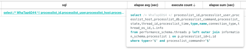
You can preview the query statement by moving the mouse pointer to the sql column in the search results list.

See query details

If you select query column from the searched result list, the SQL details window appears.

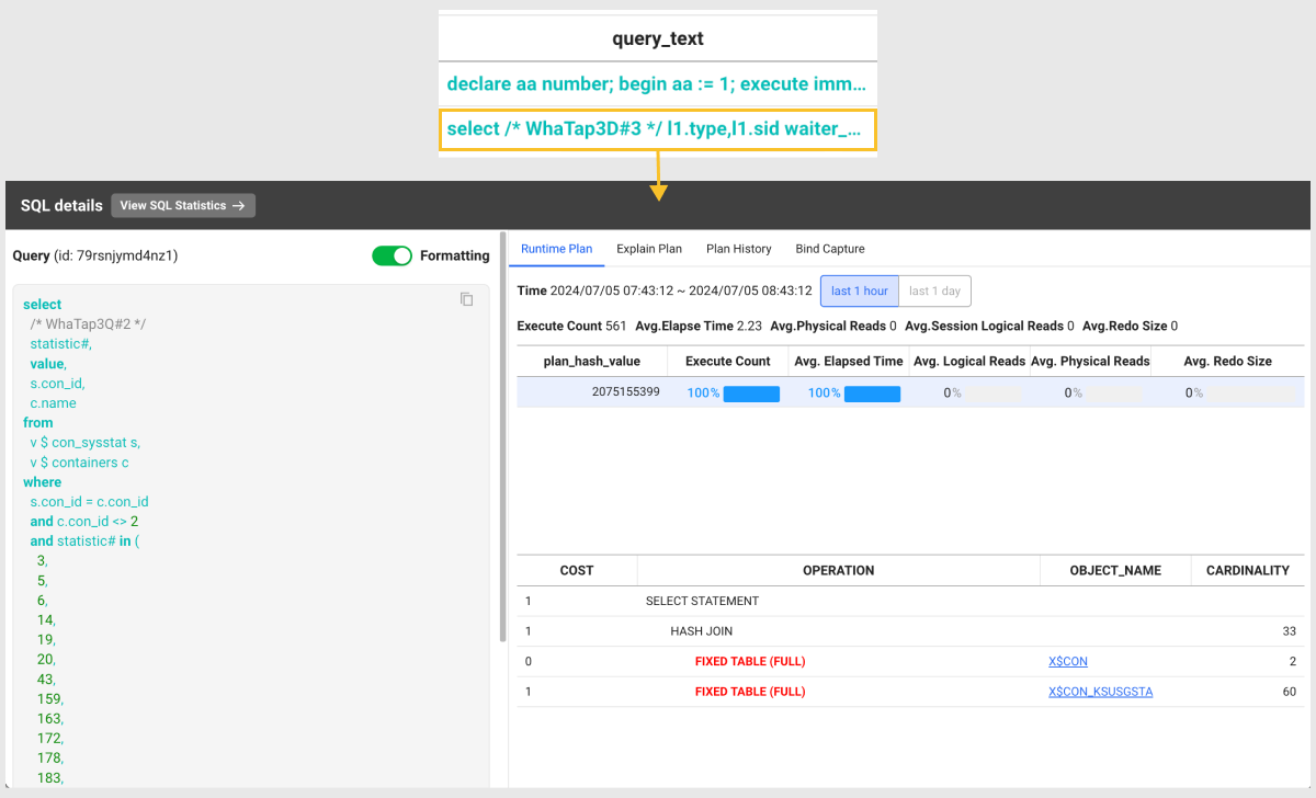
Click the View SQL Statistics → button to navigate to the SQL statistics menu, where you can view the statistical information related to the SQL query.

• Trend: Provides a comprehensive analysis of the execution time, I/O, and wait events of a specific SQL to quickly identify performance bottlenecks.
• Runtime Plan: Provides the execution plan and runtime information of the selected SQL query, including execution count, average execution time, and average physical reads.
• Explain Plan: Displays the execution plan predicted by the optimizer, showing cost, operations, object names, cardinality, and more.
• Plan History: Allows you to review the execution plan history of SQL queries executed in the database.
• Bind Capture: Displays the bind variables used in SQL queries executed in the database, allowing you to check the actual query execution contents.
  These are not real-time bind values but those captured in the database (v$sql_bind_capture).

Checking Bind Capture values

The bind values on the Bind Capture tab are masked by default. They can contain actual customer data such as resident registration numbers or account numbers, so query permission alone is no longer enough to see them.

The list itself is queried without the parameter key, because the collection time, variable name, and data type are not sensitive information. Only the value column is masked with ******.

Column	Description
time	Collection time
last_captured	The time the database last captured the bind value
name	Bind variable name
value	Bind value. Shown as ****** before decryption
datatype	Bind variable data type
child_number	Child cursor number

To check the values, follow these steps.

1. Click the lock button at the top right of the Bind Capture tab.

2. When the Check decryption key window appears, enter the parameter key. You can find the parameter key in the paramkey.txt file in the agent installation path.

3. Click the Confirm button.

If the key is correct, the window closes and the value column is filled with the actual values. Some rows may still show a dash (-) after decryption; this means the agent could not capture the value of that variable. The notation differs so that it can be distinguished from the masked state (******).

Note

If the lock button is not visible

The lock button does not appear for accounts without the sensitive information query (SECURITY_READ) permission. Contact your project administrator about permissions.

Caution

If you enter the wrong key

The message "Invalid parameter key." appears below the input field along with guidance to check paramkey.txt, and the window does not close. The reason for failure is not shown in more detail so that the key value carried in the request is not exposed on screen.

If the parameter key was changed during the query period, only some rows are filled, along with the message "The parameter key was changed during the query period, so some values were not decrypted."

A decryption query returns up to 500 rows at a time. If the limit is reached, more values may have been truncated.

Trend Tab

The top chart visualizes the trends of Elapsed Time, I/O, and Wait Time over time. The bottom statistics table provides a side-by-side comparison of cumulative execution statistics, Wait Class ratios, and major Wait Events.

Elapsed Time

Displays the total of CPU time, Wait Class time, and Idle time for the selected interval.

Example:

• CPU Time: Time actually spent using the CPU for SQL execution
• Scheduler: Time the session waited for CPU
• Idle: Time spent idle or waiting without execution (quickly see which factor consumed the most time)

Elapsed Time Trend

Shows the trend of average Elapsed Time and Execution Count aggregated in 5-minute intervals (1-minute intervals if under 3 hours).

This helps quickly identify performance degradation by checking if Elapsed Time spiked or if response time increased compared to execution count.

I/O Trend

Displays Logical Reads and Physical Reads during query execution in 5-minute intervals (1-minute intervals if under 3 hours).

• Logical Reads: Number of times data was read from the buffer cache
• Physical Reads: Number of times data was read directly from disk, allowing you to assess cache efficiency and I/O bottlenecks

Wait Time Trend

Displays the Wait Event times during query execution by time interval.

If Wait Time spikes at a certain point, it indicates DB resource contention or I/O delays. You can trace which events (lock, I/O, parallelism, etc.) caused the bottleneck.

Total Statistics

Shows cumulative SQL execution statistics for the selected interval.

Example:

• sorts(rows): Total number of sorted rows
• session logical reads: Number of session logical reads
• table scan blocks gotten: Number of blocks read during table scans
• elapsed_time: Total elapsed time
  → Provides aggregated data on how SQL execution used resources

Total Wait Classes

Displays the total Wait Time aggregated by Wait Class during SQL execution.
The higher the time for a particular Wait Class, the more likely it is the bottleneck.

Example: Idle, Scheduler, User I/O, Concurrency, etc.

Top Wait Events

Shows the top detailed Wait Events that occurred during the selected interval.
Provides more fine-grained detail than Wait Classes to identify which events most impacted performance.

Example: PX Deq: Execution Msg, resmgr:cpu quantum, direct path read, etc.

Checking the chart details

Data is fetched at different intervals depending on the query time. The available time ranges are provided in units of 1 minute (m1), 5 minutes (m5), and 1 hour (h1). To change back to the recent time, click the icon. Data is automatically adjusted according to the set time.

Detailed charts have data cycles that differ depending on the query time, just like trend charts. You can adjust the query time range by dragging.

Checking the information details

When the bar graph is selected in the chart, the Session detail window appears where you can check statistical data for 5 minutes. The list of SQL executions appears for the selected time. When an item is selected, it goes to the Instance monitoring menu with a new window.

In Instance monitoring, you can check active sessions in the table and trends of various metrics in the selected time zone.

Filtering the searched results

Adding the filter conditions

1. In the Filter option, click .

2. In Filter key, select a desired filtering criteria.

   • If the value of the selected item is text, you can select any of Includes (blue) and Excludes (red).

     

   • If the value of the selected item is number, you can select any condition of == (equal to), >= (greater than or equal to), and <= (less than or equal to).

3. In Condition, select a condition.

4. Enter a string or number to match the condition.

5. Select Apply.

Note

Adding and Deleting Filter Conditions

• To add a filtering condition, click the Add button and repeat steps 1 ~ 5. Added conditions are applied using the AND (&&) operator.

• To delete specific conditions while adding, click the button on the right side of the filter condition. To delete all conditions, click the Delete All button.

• To quickly remove all applied conditions from the Filter option, click the button.

• The default setting is to exclude if sqlText contains 'WhaTap'.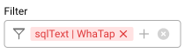

  

Modifying the filter conditions

1. Click the applied item in the Filter option at the top of the screen.

2. In the Edit filter window, edit the desired item and click the Apply button.

Setting the table columns

You can hide the table header columns or add any of them. You can also change the column order. Select .

Note

• After configuration, select Confirm to apply the settings in the table.

• In the search bar, enter text to search the desired columns. Only the columns that meet the entered text are displayed.

• Images may differ depending on the product, project, or menu.

Adding columns

From the list, select the items to add as table header columns. To select all items, select Select All.

Deleting columns

From the list, unselect the columns to delete. Alternatively, select on the right of the item to delete from the list.

Changing the column order

Drag an item to reposition from the list, and then move it to the desired position.

Initializing the configuration

To cancel all changes and reset them, select Initialized.