SQL Plan analysis

Home > Select Project > Analysis > SQL Analysis

It provides useful data for diagnosing performance issues by analyzing SQL statements executed in the database.
SQL Plan Analysis consists of the Access Statistics tab and the Plan Change History tab.

Access Statistics

The Access Statistics tab combines the execution plan history with SQL statistics to narrow down which SQL reads which tables in what way, and which of them to tune first. You can pick an unusual period from a long-range trend, drill down to the SQL list for that period, and follow through to the execution plan and per-object contribution of the SQL you choose — all on one screen. It is aimed at DBAs choosing SQL tuning targets on Oracle and Oracle Pro instances.

In other words, the screen has changed from counting Full Scan occurrences to narrowing down what the heavy SQL reads and how.

Caution

The screen has been completely restructured

The previous layout with the two charts Access Count and Operation Count is no longer provided. The trend chart has been merged into a single chart whose metric you can switch, and the Access Type summary, SQL list, execution plan, and object summary panels are placed below it.

Panel titles, table column headers, and option button labels are shown in English regardless of the screen language setting. Only some guidance texts and the funnel labels follow the screen language.

Screen layout

Block	Description
Query conditions	Set the period, instance, filters, and aggregation options as one set, then search
SQL Count trend	Shows the whole period as time-bucket bars. Drag the bars to specify the analysis range
Access Type Summary	SQL count, execution count, and share per Access Type in the analysis range
Access Type by SQL	List of Access Type composition and performance metrics per SQL
Execution Plan	Execution plan tree of the SQL selected in the list
Object Summary	Summary per object read by the selected SQL

Note

The query period and the analysis range are different

The trend chart shows the whole query period as an aggregate, while the list, execution plan, and object summary below it query only the analysis range specified on the chart as raw rows. The structure is split because receiving up to three months of execution plan steps at once would not be a manageable response.

When you first enter the screen, the analysis range is set to the most recent bucket. To widen it, drag a range on the chart, or select the full-period button in the header of the Access Type by SQL panel.

Setting the query conditions

1. Go to the Access Statistics tab in Analysis > SQL Plan Analysis.

2. Select the query period in the Time option. The default is one day, and you can specify up to three months (91 days).

3. Select the instance to query in the Instance option.

4. If needed, add conditions in the Filter option. When you first enter, the condition Access Type = TABLE ACCESS FULL is already applied.

5. Use the Exclude system objects switch to decide whether to exclude system object queries from the list. It is on by default.

6. Click the button.

Note

The period, instance, filter, and aggregation options are one set, so they are applied together only when you click the search button. In contrast, the display controls of the Access Type by SQL panel (sort criterion, number of rows, thresholds, aggregation basis, and column settings) only recalculate the data already received, so they are applied as soon as you select them.

Filter conditions

Key	Description
Access Type	Access method in the execution plan. For example, TABLE ACCESS FULL
Owner	Schema that owns the object
Object Name	Object name

Conditions support two operators: equal (=) and not equal (!=). Using not equal lets you exclude a specific schema or object from the list.

Filters apply at the SQL level, not at the execution plan step level. If an SQL has even one step matching the condition, all steps of that SQL remain in the list. Applying them per step would remove the other steps and distort the composition ratio.

Excluding system objects

This excludes queries that read only dictionary schemas such as SYS, SYSTEM, and XDB, and objects with the X$, V$, or DBA_ prefix. It regards a query that touches no user object as recursive SQL, so it is not a complete judgment. It is on by default to prevent dictionary queries such as FIXED TABLE FULL from hiding user SQL.

Viewing the SQL Count trend

The two options in the chart header determine what you see and at what resolution.

Option	Value	Description
Metric	SQL Count · Executions · Elapsed	The metric the bars represent. The default is SQL Count
Interval	Hour · Day · Week	The time width contained in one bar

Selecting a Metric also changes the panel title. The selected Access Type is drawn on top of the full bars without reducing the population, so you can read the share of that type against the whole as is.

Note

Interval Hour can be selected only up to 7 days

If the query period exceeds seven days, the Hour button is disabled and the message "Cannot be viewed by hour for queries longer than 7 days" is displayed. Seven days means 168 time buckets, which can still be selected by hand, but beyond that it becomes hard to pick a range.

If you have not selected an Interval, or the value cannot be used for the current query period, the period determines the unit: Hour for two days or less, and Day for longer.

Specify the analysis range by clicking a bar or dragging across several bars. The specified range becomes the query scope of the three panels below.

Reading the Access Type Summary

It aggregates how much each Access Type was used in the analysis range.

Column	Description
Access Type	Access method in the execution plan
SQL Count	Number of SQL statements that used that access method
Executions	Total execution count
Share	Share based on execution count

If one SQL uses both a Full Scan and a Range Scan, it is added to both. That is, Share reads as "the portion taken by SQL that uses this access method", and the total can exceed 100%.

Working with the Access Type by SQL list

The list consists of one row per combination of SQL and execution plan (sql_id + plan_hash_value).

Display controls

Option	Default	Description
Sort criterion	Logical IO	Choose from Logical IO, Elapsed, Executions, LIO / exec, Full Steps
Number of rows	Top 50	From Top 20 to Top 1,000, or No limit
Minimum executions	0	Lower bound for execution count
Minimum LIO per execution	0	Lower bound for logical reads per execution
Basis	Range Total	Basis for aggregating metrics. Range Total sums the range, Latest Plan uses the latest execution plan

The two thresholds default to 0 to prevent some SQL from being silently dropped as soon as you enter the screen. The list length is already bounded by the number of rows, so use the thresholds as a tool to narrow things down when you need to.

Funnel display

The panel header shows where and by how much the list was reduced, in three steps.

Step	Description
In range	Number of SQL statements that fell in the analysis range
Passed conditions	Number of SQL statements that passed the filters and thresholds
Displayed	Number of rows actually drawn in the table

The first two values are SQL counts and the last is a row count. The units differ because a row is a combination of SQL and execution plan.

Column layout

Group	Column	Description
SQL	sql_id · plan_hash_value · query_text	SQL identifier and statement
Composition	Steps · Breakdown	Number of execution plan steps and the Access Type composition bar
Performance	Executions · LIO/exec · Elapsed/exec(s)	Execution count and load per execution

Access Type columns are divided into four tiers by risk: High Risk, Caution, Normal, and Hidden. You can choose which types to display in the column settings, and the remaining steps that do not match the definition table are collected in the Others column.

The Access Types enabled by default are as follows.

Access Type	Tier
TABLE ACCESS FULL	High Risk
PARTITION RANGE ALL	High Risk
INDEX SKIP SCAN	Caution
INDEX FAST FULL SCAN	Caution
INDEX FULL SCAN	Caution
INDEX RANGE SCAN	Normal
INDEX UNIQUE SCAN	Normal
TABLE ACCESS BY INDEX ROWID	Normal

TABLE ACCESS STORAGE FULL, BITMAP INDEX, MAT_VIEW ACCESS, HASH JOIN, NESTED LOOPS, MERGE JOIN, and FIXED TABLE FULL are hidden by default and can be enabled in the column settings.

Viewing the selected SQL in detail

When you select a row in the list, the two panels below are filled with the content of that SQL.

Execution Plan

Column	Description
Operation	Execution plan step
Object	Object being accessed
Cost	Cost assigned by the optimizer

Object Summary

Column	Description
Object	Object name
Access Type	How that object is read
Index	Index used
Cost Share	Share of the total cost

The table is first sorted by Cost Share in descending order so that the object contributing most to the load comes first. You can change the sort by clicking a column header.

Good to know

• LIO (Logical IO) can be measured only at the SQL level. Values broken down by step are not provided, so Access Type Summary has no LIO contribution column.

• If you select several Access Types on the trend chart, the sum of the overlaid values can exceed the full bar. This is because one SQL uses several types together, and the screen clips the display so that it does not extend beyond the bar.

• The counts in the chart range and the number of rows in the list can differ by a few. The chart comes from an aggregate query while the list comes from the same data with system and recursive exclusion conditions applied, and the screen aligns the numbers with the list that users actually compare against.

View SQL Details

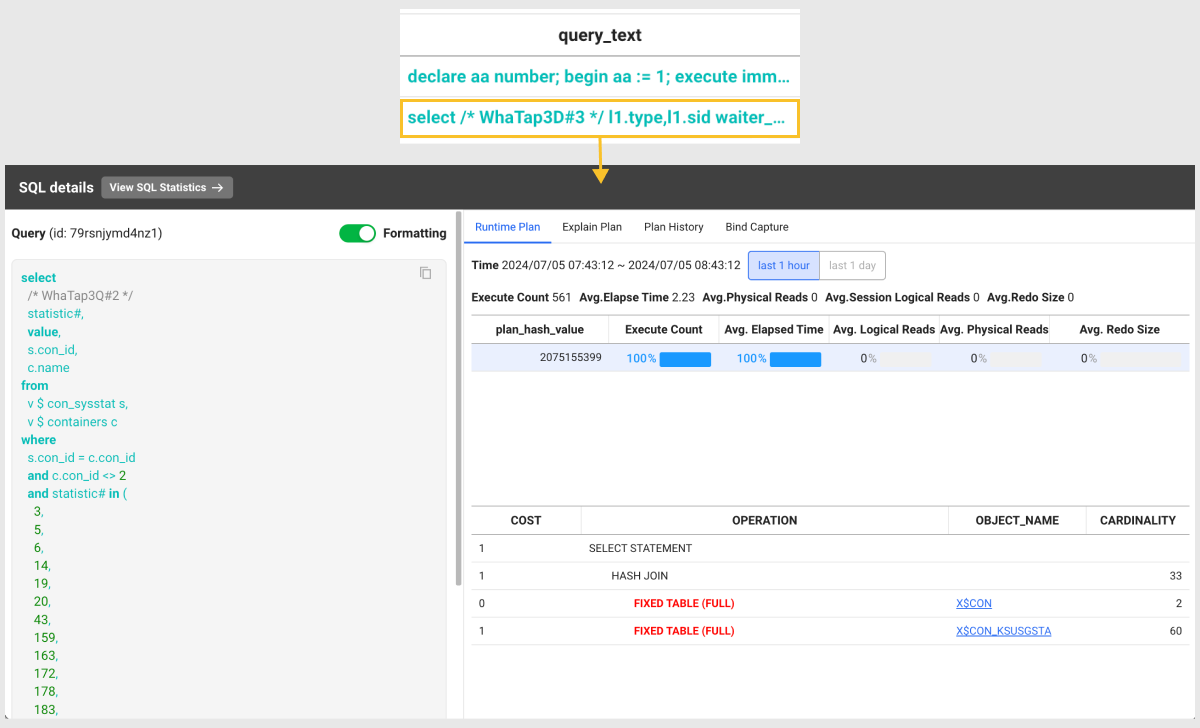
If you select the query column from the SQL list at the bottom of the screen, the SQL details window appears. You can check the SQL query statements and plan information.

Click the View SQL Statistics → button to move to SQL statistics,
where you can view statistical information related to the selected SQL query.

• Runtime Plan: It provides the execution plan and runtime information for a selected SQL query. It provides the information details such as execution count, average execution time, and average physical reads.

• Explain Plan: It displays the execution plan predicted by the optimizer. It provides information such as cost, job, object name, and cardinality.

• Plan History: You can check the history of the execution plans of the SQL queries executed in the database.

• Bind Capture: You can check the bind variables used in SQL queries executed in the database. This allows you to see actual content of query executions.

  Note

  This is a value captured in the database (v$sql_bind_capture), not a bind value executed in real time.

• Trend: You can check the trend of execution metrics for the selected SQL in a time-series chart and a table. It shows changes in execution time, average metrics per execution, and parse counts (total and hard) in chronological order.

  Note

  The set of metrics shown on the Trend tab differs between Oracle and Oracle Pro.

Checking Bind Capture values

The bind values on the Bind Capture tab are masked by default. They can contain actual customer data such as resident registration numbers or account numbers, so query permission alone is no longer enough to see them.

The list itself is queried without the parameter key, because the collection time, variable name, and data type are not sensitive information. Only the value column is masked with ******.

Column	Description
time	Collection time
last_captured	The time the database last captured the bind value
name	Bind variable name
value	Bind value. Shown as ****** before decryption
datatype	Bind variable data type
child_number	Child cursor number

To check the values, follow these steps.

1. Click the lock button at the top right of the Bind Capture tab.

2. When the Check decryption key window appears, enter the parameter key. You can find the parameter key in the paramkey.txt file in the agent installation path.

3. Click the Confirm button.

If the key is correct, the window closes and the value column is filled with the actual values. Some rows may still show a dash (-) after decryption; this means the agent could not capture the value of that variable. The notation differs so that it can be distinguished from the masked state (******).

Note

If the lock button is not visible

The lock button does not appear for accounts without the sensitive information query (SECURITY_READ) permission. Contact your project administrator about permissions.

Caution

If you enter the wrong key

The message "Invalid parameter key." appears below the input field along with guidance to check paramkey.txt, and the window does not close. The reason for failure is not shown in more detail so that the key value carried in the request is not exposed on screen.

If the parameter key was changed during the query period, only some rows are filled, along with the message "The parameter key was changed during the query period, so some values were not decrypted."

A decryption query returns up to 500 rows at a time. If the limit is reached, more values may have been truncated.

AI Tuning Guide

The AI Tuning Guide analyzes SQL queries, plans, and statistical information to diagnose performance issues and suggest optimization strategies.
It helps developers and DBAs quickly identify bottlenecks and improve performance through efficient SQL optimization.

Caution

Usage Conditions and Notes

For PostgreSQL, MySQL, and SQL Server, query plan retrieval is required.
If the plan is not retrieved, the AI Tuning Guide icon appears as (disabled), and the feature cannot be used.

• Please note that AI-generated results are based on automated analysis and may not be 100% accurate.

1. Click the SQL you want to analyze and diagnose to move to the SQL details screen.

2. On the SQL details screen, click the AI Tuning Guide icon at the bottom right to start the AI analysis.

3. Review the AI analysis results.

   Result Item	Description
   Query Plan and Summary	Provides the purpose and execution summary of the query. Analyzes execution count, cumulative execution time, and overall database load ratio to assess the query’s impact on system performance.
   Performance Analysis	Provides performance scores and diagnostic results based on overall analysis. Analyzes detailed resource usage such as CPU, disk, cache hit rate, and wait time to visually identify bottleneck areas during query execution.
   Key Issues Found	Summarizes detected major issues.
   Optimization Recommendations	Suggests optimized queries based on identified issues.

Plan Change History

In the Plan Change History tab, even if the SQL ID is the same, performance can be affected when the execution plan changes.
By detecting and monitoring plan changes made by the optimizer, you can prevent unnecessary changes and maintain consistent SQL performance.

1. Go to the Plan Change Historys tab in Analysis > SQL Plan Analysis.

2. Select the query time and instance.

3. Set the Time and Instance options, then click the button.

4. In the Plan Change Count section, select a specific time period to view the list of plan changes that occurred during that time.

   • Plan Change Count section: A bar chart showing the number of plan changes that occurred by time period.

Checking the plan change details

1. In the Plan Change Historys tab of SQL Plan Analysis, click a specific change item from the list.

2. In the Query section, details before and after the plan change are displayed.
   Compare the differences to identify the cause of performance changes.

   • In the Query section, click the button in the upper-right corner to view the section in a new window.

3. To close the Query section, click the button in the upper-right corner.

Filtering the searched results

You can filter the query results based on the following criteria.

• sql_id

• sql_hash_value

• after_plan_hash_value

• before_plan_hash_value

Adding the filter conditions

1. In the Filter option, click .

2. In Filter key, select a desired filtering criteria.

   • If the value of the selected item is text, you can select any of Includes (blue) and Excludes (red).

     

   • If the value of the selected item is number, you can select any condition of == (equal to), >= (greater than or equal to), and <= (less than or equal to).

3. In Condition, select a condition.

4. Enter a string or number to match the condition.

5. Select Apply.

Note

Adding and Deleting Filter Conditions

• To add a filtering condition, click the Add button and repeat steps 1 ~ 5. Added conditions are applied using the AND (&&) operator.

• To delete specific conditions while adding, click the button on the right side of the filter condition. To delete all conditions, click the Delete All button.

• To quickly remove all applied conditions from the Filter option, click the button.

Modifying the filter conditions

1. Click the applied item in the Filter option at the top of the screen.

2. In the Edit filter window, edit the desired item and click the Apply button.